Fit a Mean Parametrized Conway-Maxwell Poisson Generalized Linear Model
Source:R/glm.cmp.R
glm.cmp.RdThe function glm.cmp is used to fit a mean parametrized Conway-Maxwell Poisson
generalized linear model with a log-link by using Fisher Scoring iteration.
glm.cmp(
  formula,
  formula_nu = NULL,
  data,
  offset = NULL,
  subset,
  na.action,
  betastart = NULL,
  gammastart = NULL,
  lambdalb = 1e-10,
  lambdaub = 1000,
  maxlambdaiter = 1000,
  tol = 1e-06,
  contrasts_mu = NULL,
  contrasts_nu = NULL
)
Arguments
- formula
an object of class 'formula': a symbolic description of the model to be fitted to the mean via log-link.
- formula_nu
an optional object of class 'formula': a symbolic description of the model to be fitted to the dispersion via log-link.
- data
an optional data frame containing the variables in the model
- offset
this can be used to specify an a priori known component to be included in the linear predictor for mean during fitting. This should be
NULLor a numeric vector of length equal to the number of cases.- subset
an optional vector specifying a subset of observations to be used in the fitting process.
- na.action
a function which indicates what should happen when the data contain NAs. The default is set by the na.action setting of options, and is na.fail if that is unset. The ‘factory-fresh’ default is na.omit. Another possible value is NULL, no action. Value na.exclude can be useful.
- betastart
starting values for the parameters in the linear predictor for mu.
- gammastart
starting values for the parameters in the linear predictor for nu.
- lambdalb, lambdaub
numeric: the lower and upper end points for the interval to be searched for lambda(s). The default value for lambdaub should be sufficient for small to moderate size nu. If nu is large and required a larger
lambdaub, the algorithm will scale uplambdaubaccordingly.- maxlambdaiter
numeric: the maximum number of iterations allowed to solve for lambda(s).
- tol
numeric: the convergence threshold. A lambda is said to satisfy the mean constraint if the absolute difference between the calculated mean and a fitted values is less than tol.
- contrasts_mu, contrasts_nu
optional lists. See the contrasts.arg of model.matrix.default.
Value
A fitted model object of class cmp similar to one obtained from glmor glm.nb.
The function summary (i.e., summary.cmp) can be used to obtain
and print a summary of the results.
The functions plot (i.e., plot.cmp) and
gg_plot can be used to produce a range
of diagnostic plots.
The generic assessor functions coef (i.e., coef.cmp),
logLik (i.e., logLik.cmp)
fitted (i.e., fitted.cmp),
nobs (i.e., nobs.cmp),
AIC (i.e., AIC.cmp) and
residuals (i.e., residuals.cmp)
can be used to extract various useful features of the value
returned by glm.cmp.
The functions LRTnu and cmplrtest can be used to perform a likelihood ratio
chi-squared test for nu = 1 and for nested COM-Poisson model respectively.
An object class 'glm.cmp' is a list containing at least the following components:
- coefficients
a named vector of coefficients
- coefficients_beta
a named vector of mean coefficients
- coefficients_gamma
a named vector of dispersion coefficients
- se_beta
approximate standard errors (using observed rather than expected information) for mean coefficients
- se_gamma
approximate standard errors (using observed rather than expected information) for dispersion coefficients
- residuals
the response residuals (i.e., observed-fitted)
- fitted_values
the fitted mean values
- rank_mu
the numeric rank of the fitted linear model for mean
- rank_nu
the numeric rank of the fitted linear model for dispersion
- linear_predictors
the linear fit for mean on log scale
- df_residuals
the residuals degrees of freedom
- df_null
the residual degrees of freedom for the null model
- null_deviance
The deviance for the null model. The null model will include only the intercept.
- deviance; residual_deviance
The residual deviance of the model
- y
the
yvector used.- x
the model matrix for mean
- s
the model matrix for dispersion
- model_mu
the model frame for mu
- model_nu
the model frame for nu
- call
the matched call
- formula
the formula supplied for mean
- formula_nu
the formula supplied for dispersion
- terms_mu
the
termsobject used for mean- terms_nu
the
termsobject used for dispersion- data
the
dataargument- offset
the
offsetvector used- lambdaub
the final
lambdaubused
Details
Fit a mean-parametrized COM-Poisson regression using maximum likelihood estimation via an iterative Fisher Scoring algorithm.
Currently, the COM-Poisson regression model allows constant dispersion and regression being linked to the dispersion parameter i.e. varying dispersion.
For the constant dispersion model, the model is
$$Y_i \sim CMP(\mu_i, \nu),$$
where
$$E(Y_i) = \mu_i = exp(x_i^{\top} \beta),$$
and \(\nu > 0\) is the dispersion parameter.
The fitted COM-Poisson distribution is over- or under-dispersed if \(\nu < 1\) and \(\nu > 1\) respectively.
For the varying dispersion model, the model is
$$Y_i \sim CMP(\mu_i, \nu_i),$$
where
$$E(Y_i) = \mu_i = exp(x_i^{\top} \beta),$$
and dispersion parameters are model via
$$\nu_i = exp(s_i^{\top} \gamma),$$
where \(x_i\) and \(s_i\) are some covariates.
References
Fung, T., Alwan, A., Wishart, J. and Huang, A. (2020). mpcmp: Mean-parametrized
Conway-Maxwell Poisson Regression. R package version 0.3.4.
Huang, A. (2017). Mean-parametrized Conway-Maxwell-Poisson regression models for dispersed counts. Statistical Modelling 17, 359--380.
See also
summary.cmp, autoplot.cmp, plot.cmp, fitted.cmp,
residuals.cmp and LRTnu.
Additional examples may be found in fish,
takeoverbids, cottonbolls.
Examples
### Huang (2017) Page 368--370: Overdispersed Attendance data
data(attendance)
M.attendance <- glm.cmp(daysabs ~ gender + math + prog, data = attendance)
M.attendance
#>
#> Call: glm.cmp(formula = daysabs ~ gender + math + prog, data = attendance)
#>
#> Linear Model Coefficients:
#> (Intercept) gendermale math progAcademic progVocational
#> 2.714600 -0.214720 -0.006323 -0.425320 -1.253900
#>
#> Dispersion (nu): 0.0202
#> Degrees of Freedom: 313 Total (i.e. Null); 309 Residual
#> Null Deviance: 455.8327
#> Residual Deviance:
#> AIC: 1739.026
#>
summary(M.attendance)
#>
#> Call: glm.cmp(formula = daysabs ~ gender + math + prog, data = attendance)
#>
#> Deviance Residuals:
#> Min 1Q Median 3Q Max
#> -2.1925 -1.1166 -0.3973 0.2964 2.8154
#>
#> Linear Model Coefficients:
#> Estimate Std.Err Z value Pr(>|z|)
#> (Intercept) 2.714645 0.190407 14.257 < 2e-16 ***
#> gendermale -0.214720 0.117148 -1.833 0.06682 .
#> math -0.006323 0.002386 -2.650 0.00804 **
#> progAcademic -0.425322 0.169525 -2.509 0.01211 *
#> progVocational -1.253896 0.189478 -6.618 3.65e-11 ***
#> ---
#> Signif. codes: 0 ‘***’ 0.001 ‘**’ 0.01 ‘*’ 0.05 ‘.’ 0.1 ‘ ’ 1
#>
#> (Dispersion parameter for Mean-CMP estimated to be 0.02024)
#>
#>
#> Null deviance: 455.83 on 313 degrees of freedom
#> Residual deviance: 377.44 on 309 degrees of freedom
#>
#> AIC: 1739.026
#>
# \donttest{
plot(M.attendance) # or autoplot(M.attendance)
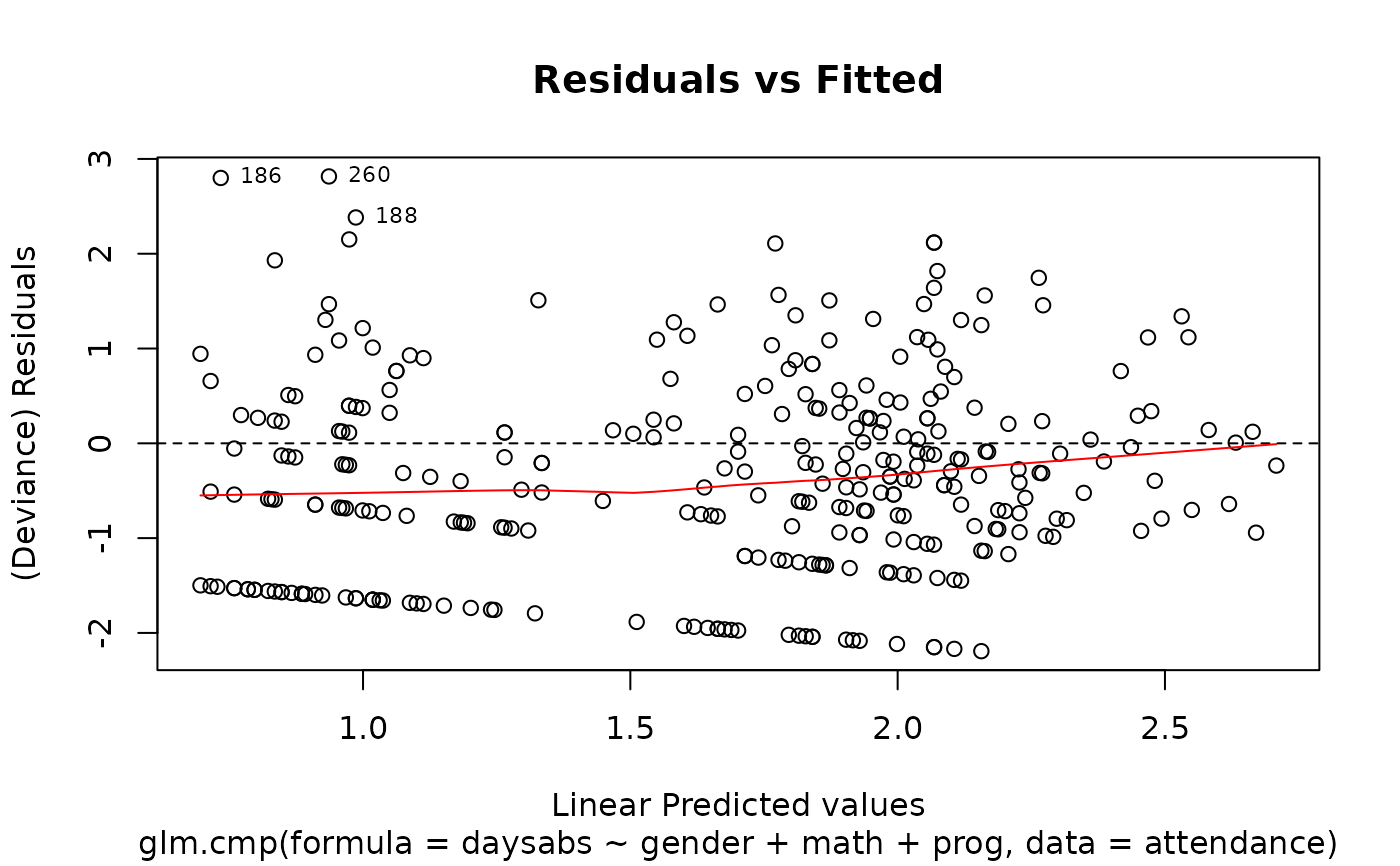
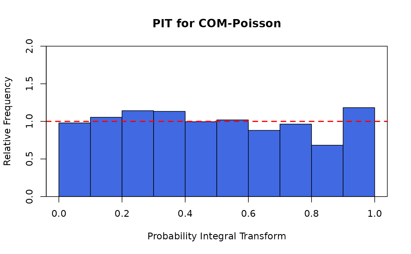
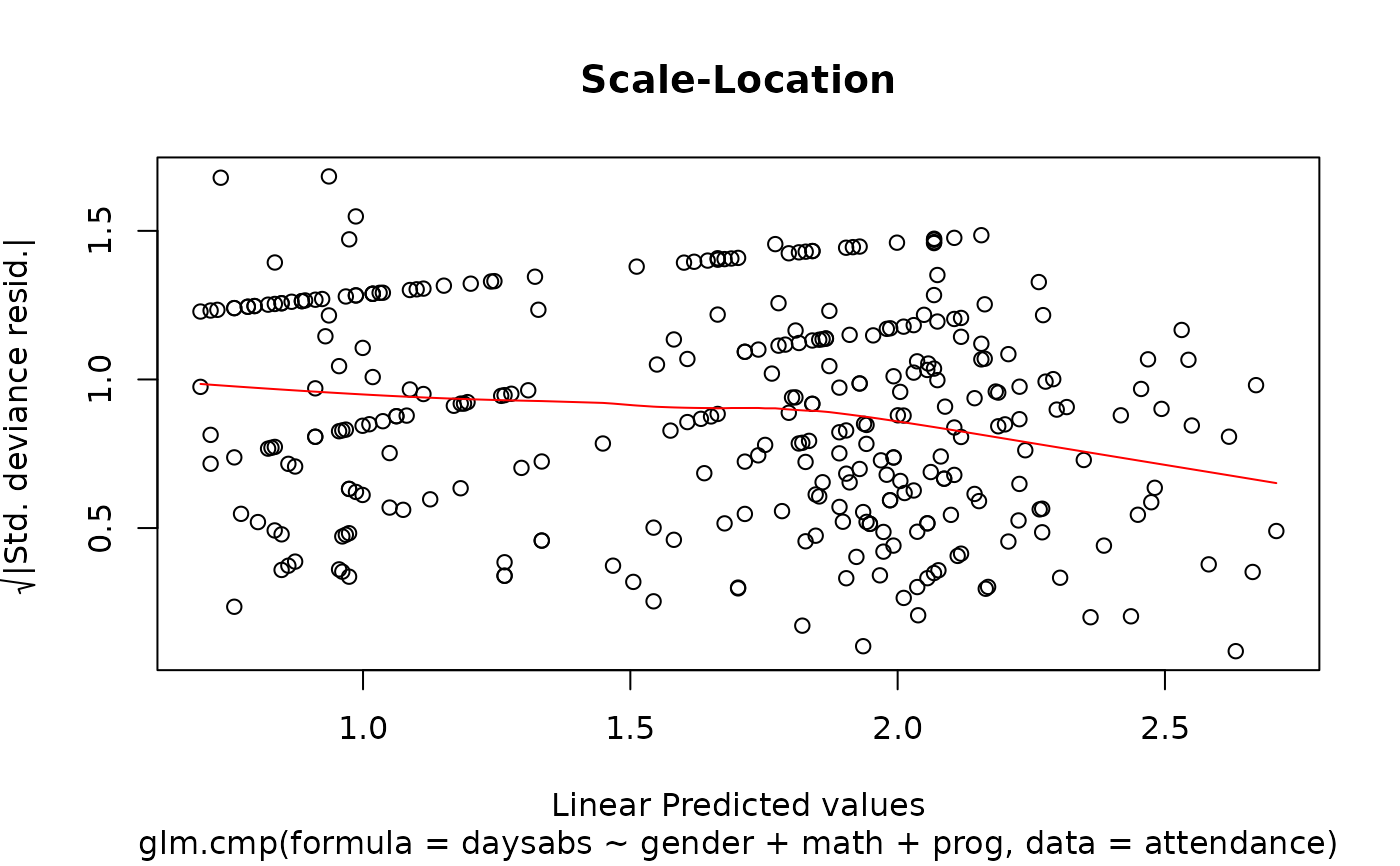
 # }
### Ribeiro et al. (2013): Varying dispersion as a function of covariates
# \donttest{
data(sitophilus)
M.sit <- glm.cmp(formula = ninsect ~ extract, formula_nu = ~extract, data = sitophilus)
summary(M.sit)
#>
#> Call: glm.cmp(formula = ninsect ~ extract, formula_nu = ~extract, data = sitophilus)
#>
#> Deviance Residuals:
#> Min 1Q Median 3Q Max
#> -2.21085 -1.16849 0.07494 0.64152 1.72653
#>
#> Mean Model Coefficients:
#> Estimate Std.Err Z value Pr(>|z|)
#> (Intercept) 3.449988 0.077974 44.245 <2e-16 ***
#> extractLeaf -0.006369 0.122139 -0.052 0.958
#> extractBranch -0.052129 0.123387 -0.422 0.673
#> extractSeed -3.354677 0.362108 -9.264 <2e-16 ***
#> ---
#> Signif. codes: 0 ‘***’ 0.001 ‘**’ 0.01 ‘*’ 0.05 ‘.’ 0.1 ‘ ’ 1
#>
#> Dispersion Model Coefficients:
#> Estimate Std.Err Z value Pr(>|z|)
#> (Intercept) -0.6652 0.4573 -1.455 0.146
#> extractLeaf -0.3831 0.6509 -0.589 0.556
#> extractBranch -0.3724 0.6514 -0.572 0.567
#> extractSeed -0.1176 1.5461 -0.076 0.939
#>
#> Null deviance: 257.211 on 39 degrees of freedom
#> Residual deviance: 41.679 on 32 degrees of freedom
#>
#> AIC: 260.8279
#>
# }
# }
### Ribeiro et al. (2013): Varying dispersion as a function of covariates
# \donttest{
data(sitophilus)
M.sit <- glm.cmp(formula = ninsect ~ extract, formula_nu = ~extract, data = sitophilus)
summary(M.sit)
#>
#> Call: glm.cmp(formula = ninsect ~ extract, formula_nu = ~extract, data = sitophilus)
#>
#> Deviance Residuals:
#> Min 1Q Median 3Q Max
#> -2.21085 -1.16849 0.07494 0.64152 1.72653
#>
#> Mean Model Coefficients:
#> Estimate Std.Err Z value Pr(>|z|)
#> (Intercept) 3.449988 0.077974 44.245 <2e-16 ***
#> extractLeaf -0.006369 0.122139 -0.052 0.958
#> extractBranch -0.052129 0.123387 -0.422 0.673
#> extractSeed -3.354677 0.362108 -9.264 <2e-16 ***
#> ---
#> Signif. codes: 0 ‘***’ 0.001 ‘**’ 0.01 ‘*’ 0.05 ‘.’ 0.1 ‘ ’ 1
#>
#> Dispersion Model Coefficients:
#> Estimate Std.Err Z value Pr(>|z|)
#> (Intercept) -0.6652 0.4573 -1.455 0.146
#> extractLeaf -0.3831 0.6509 -0.589 0.556
#> extractBranch -0.3724 0.6514 -0.572 0.567
#> extractSeed -0.1176 1.5461 -0.076 0.939
#>
#> Null deviance: 257.211 on 39 degrees of freedom
#> Residual deviance: 41.679 on 32 degrees of freedom
#>
#> AIC: 260.8279
#>
# }