Plot Diagnostic for a tsglm.izip Object

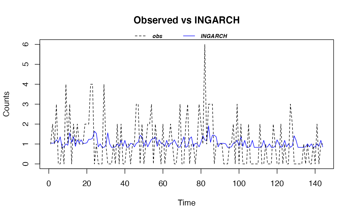
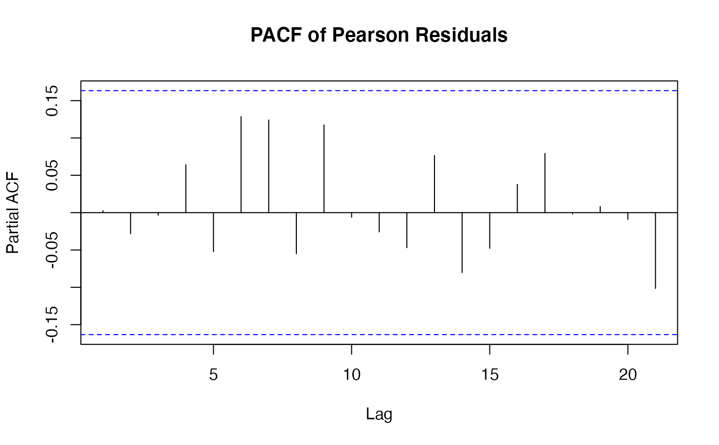
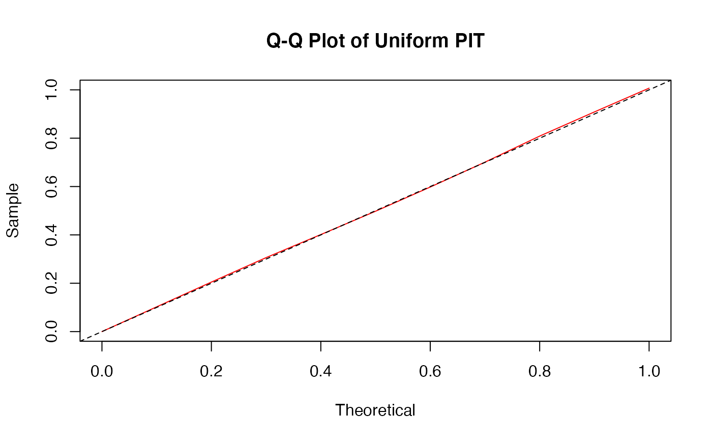
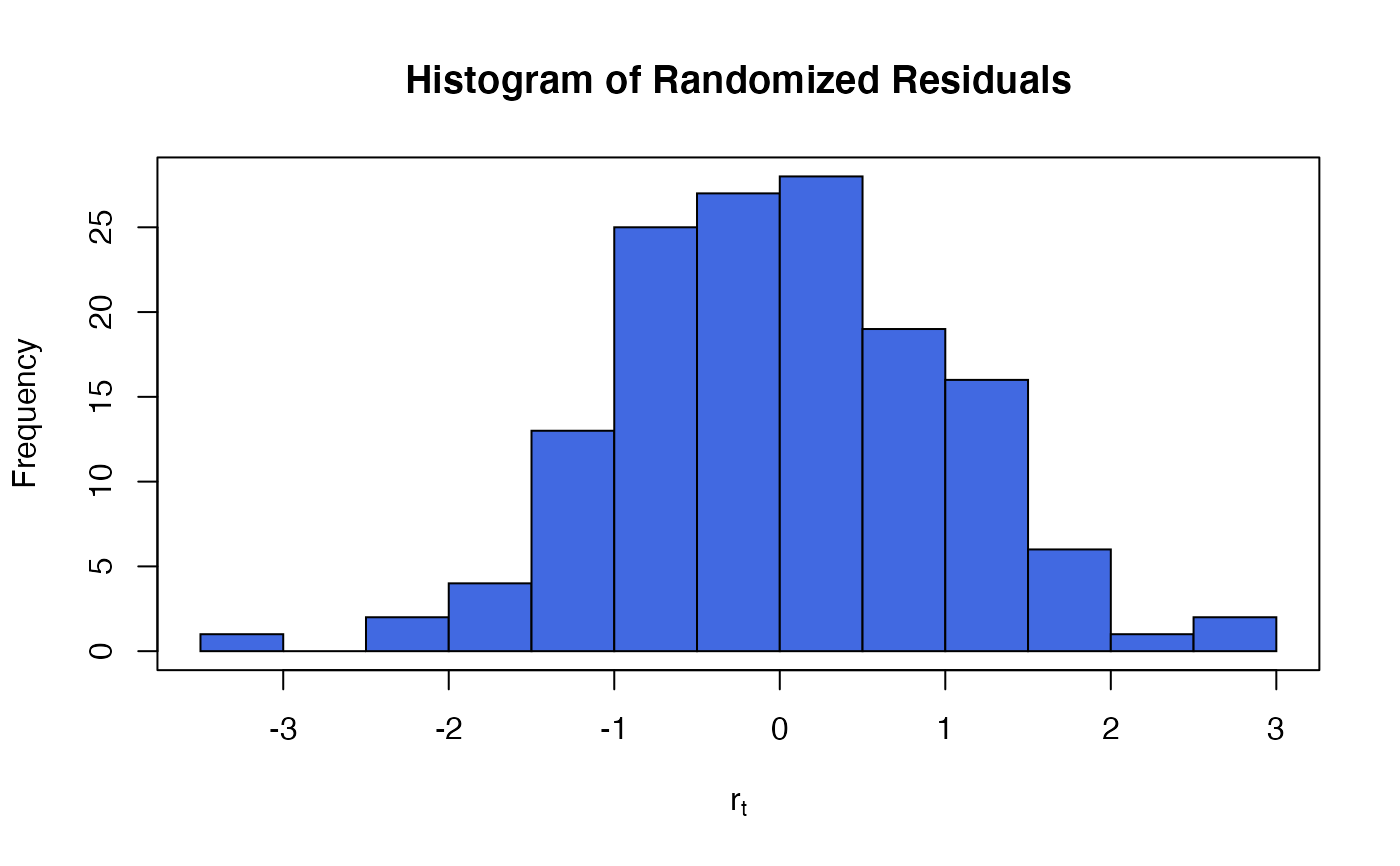
Eleven plots (selectable by which) are currently available using ggplot or graphics: a plot of observed vs fitted time series plot, an ACF plot of Pearson residuals, a PACF plot of Pearson residuals, a plot of Pearson residuals against time, a Normal Q-Q Plot of Pearson residuals, an non-randomized PIT histogram, an uniform Q-Q plot for non-randomized PIT, a histogram of normal randomized residuals, a Q-Q plot of the normal randomized residuals, 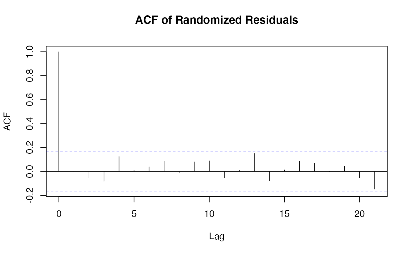an ACF plot of the normal randomized residuals 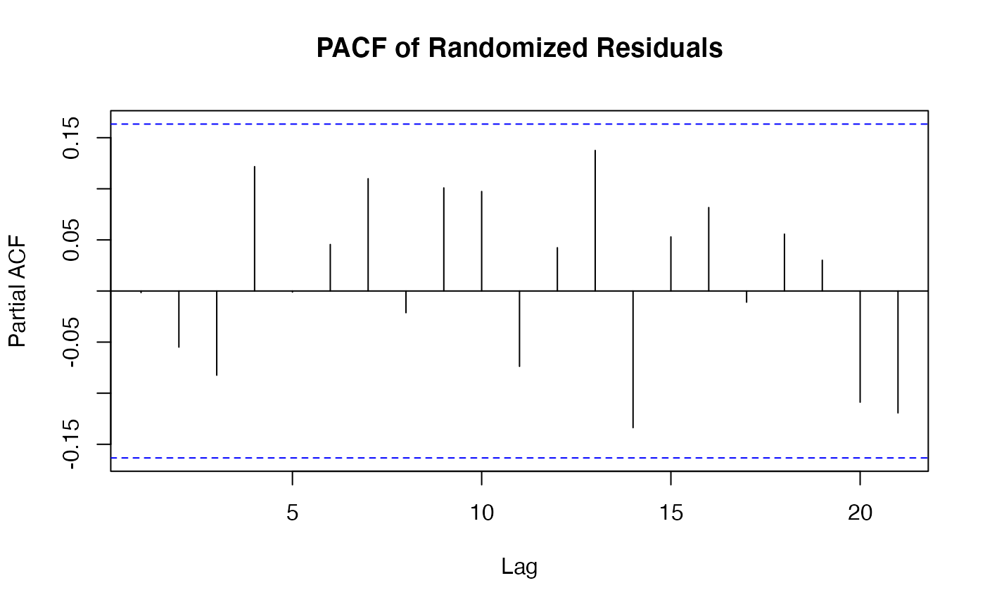a PACF plot of the normal randomized residuals

# S3 method for tsizip
plot(
  x,
  which = c(1L, 3L, 5L, 7L, 8L, 9L),
  ask = prod(par("mfcol")) < length(which) && dev.interactive(),
  bins = 10,
  ...
)

# S3 method for tsizip
autoplot(
  object,
  which = c(1L, 6L, 7L, 10L, 11L),
  bins = 10,
  ask = TRUE,
  nrow = NULL,
  ncol = NULL,
  output_as_ggplot = TRUE,
  ...
)

Arguments

x	an object class 'tsizip' object, obtained from a call to tsglm.izip
which	if a subset of plots is required, specify a subset of the numbers 1:11. See 'Details' below.
ask	logical; if TRUE, the user is asked before each plot.
bins	numeric; the number of bins shown in the PIT histogram or the PIT Q-Q plot.
...	other arguments passed to or from other methods (currently unused).
object	an object class 'tsizip' object, obtained from a call to tsglm.izip
nrow	numeric; (optional) number of rows in the plot grid.
ncol	numeric; (optional) number of columns in the plot grid.
output_as_ggplot	logical; if TRUE, the function would return a list of ggplot objects; if FALSE, the function would return an ggarrange object, which is a ggplot or a list of ggplot.

Value

A ggarrange object, which is a ggplot or a list of ggplot for autoplot.

Details

By default, 6 plots (number 1, 6, 7, 8, 10 and 11 from this list of plots) are provided for plot and 5 plots (number 1, 6, 7, 10 and 11) are provided for autoplot

There are two plots based on the non-randomized probability integral transformation (PIT) using izipPIT. These are a histogram and a uniform Q-Q plot. If the model assumption is appropriate, these plots should reflect a sample obtained from a uniform distribution.

There are also two plots based on the normal randomized residuals calculated using izipnormRandPIT. These are a histogram and a normal Q-Q plot. If the model assumption is appropriate, these plots should reflect a sample obtained from a normal distribution.

See also

izipPIT, izipnormRandPIT, and tsglm.izip.

Examples

data(arson)
M_arson <- tsglm.izip(arson ~ 1, past_mean_lags = 1, past_obs_lags = c(1, 2))
## The default plots are shown
plot(M_arson) # or autoplot(M_arson)

## The plots for the ACF and PACF of the normal randomized residuals
plot(M_arson, which = c(10, 11))
# or autoplot(M_arson, which = c(10,11))