Plot Diagnostic for a glm.izip Object

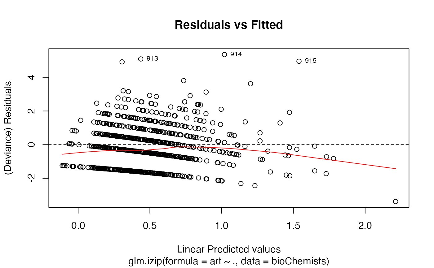
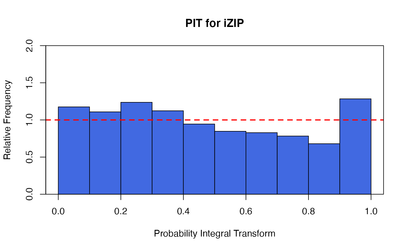
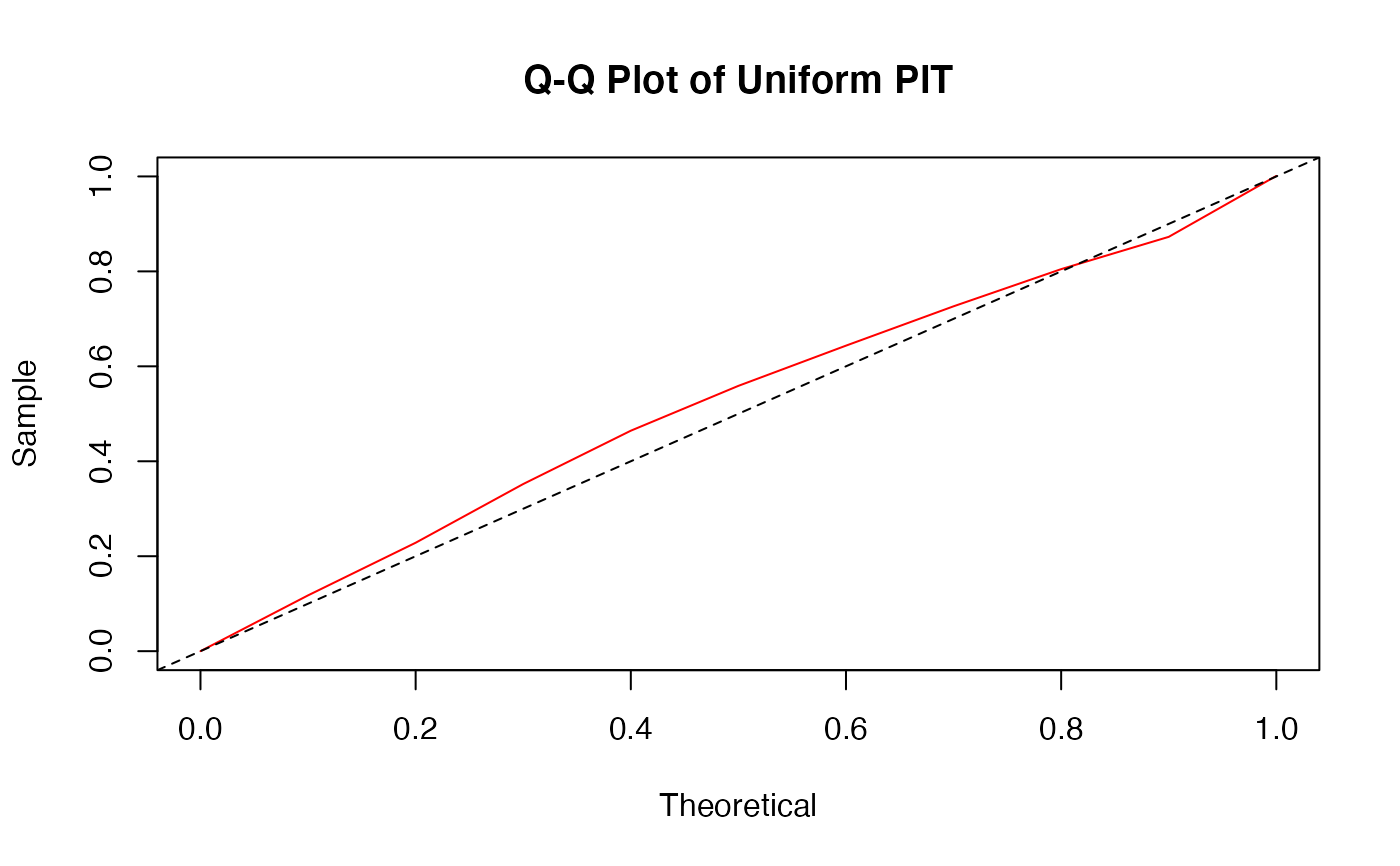
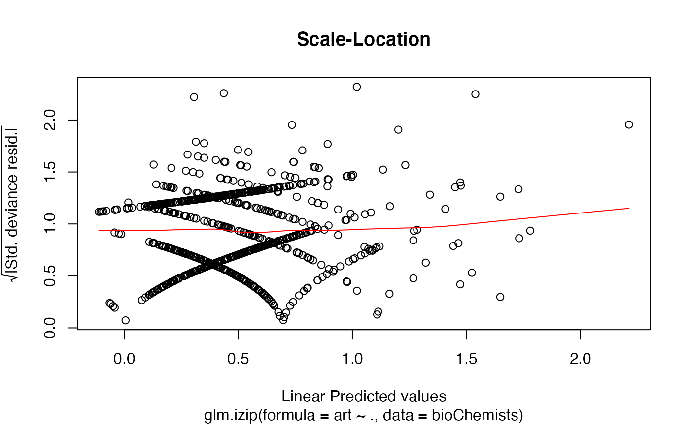
Eight plots (selectable by which) are currently available using ggplot or graphics: a plot of deviance residuals against fitted values, a non-randomized PIT histogram, a uniform Q-Q plot for non-randomized PIT, a histogram of the normal randomized residuals, a Q-Q plot of the normal randomized residuals, a Scale-Location plot of sqrt(| residuals |) against fitted values a plot of Cook's distances versus row labels 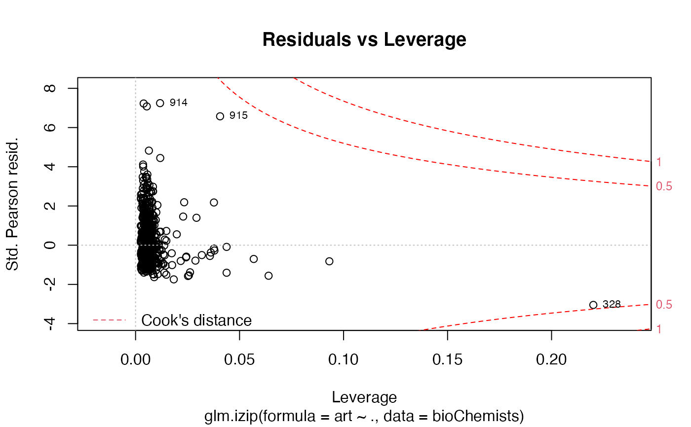a plot of pearson residuals against leverage. By default, four plots (number 1, 2, 6, and 8 from this list of plots) are provided.

# S3 method for izip
plot(
  x,
  which = c(1L, 2L, 6L, 8L),
  ask = prod(par("mfcol")) < length(which) && dev.interactive(),
  bins = 10,
  ...
)

# S3 method for izip
autoplot(
  x,
  which = c(1L, 2L, 6L, 8L),
  bins = 10,
  ask = TRUE,
  nrow = NULL,
  ncol = NULL,
  output_as_ggplot = TRUE
)

Arguments

x	an object class 'izip' object, obtained from a call to glm.izip
which	if a subset of plots is required, specify a subset of the numbers 1:8. See 'Details' below.
ask	logical; if TRUE, the user is asked before each plot.
bins	numeric; the number of bins shown in the PIT histogram or the PIT Q-Q plot.
...	other arguments passed to or from other methods (currently unused).
nrow	numeric; (optional) number of rows in the plot grid.
ncol	numeric; (optional) number of columns in the plot grid.
output_as_ggplot	logical; if TRUE, the function would return a list of ggplot objects; if FALSE, the function would return an ggarrange object, which is a ggplot or a list of ggplot.

Value

A ggarrange object, which is a ggplot or a list of ggplot for autoplot.

Details

The 'Scale-Location' plot, also called 'Spread-Location' plot, takes the square root of the absolute standardized deviance residuals (sqrt|E|) in order to diminish skewness is much less skewed than than |E| for Gaussian zero-mean E.

The 'Scale-Location' plot uses the standardized deviance residuals while the Residual-Leverage plot uses the standardized pearson residuals. They are given as \(R_i/\sqrt{1-h_{ii}}\) where \(h_{ii}\) are the diagonal entries of the hat matrix.

The Residuals-Leverage plot shows contours of equal Cook's distance for values of 0.5 and 1.

There are two plots based on the non-randomized probability integral transformation (PIT) using izipPIT. These are a histogram and a uniform Q-Q plot. If the model assumption is appropriate, these plots should reflect a sample obtained from a uniform distribution.

There are also two plots based on the normal randomized residuals calculated using izipnormRandPIT. These are a histogram and a normal Q-Q plot. If the model assumption is appropriate, these plots should reflect a sample obtained from a normal distribution.

See also

izipPIT, izipnormRandPIT, and glm.izip.

Examples

data(bioChemists)
M_bioChem <- glm.izip(art ~ ., data = bioChemists)

## The default plots are shown
plot(M_bioChem) # or autoplot(M_bioChem)

## The plots for the non-randomized PIT
plot(M_bioChem, which = c(2, 3))
# or autoplot(M_bioChem, which = c(2,3))